27.3. How to begin Wrangling: Get to know your Data!

Whenever you begin working with a new dataset, it’s essential that you get to know your data! To get started, there are a few questions to consider:

• Where did the data come from and how it was collected?

• What data types are my variables (numeric, string, date, etc)?

• Does Python recognize recognize these variables as their correct data types?

• Are there outliers in our data?

• How should we handle missing data?

The answers to these questions are just a handful of ways that may influence the approaches you take to wrangle your data.

Note

Data wrangling may also be referred to as data cleaning. By wrangling our data, we help ensure that it will be clean for later analysis.

Case Study of Data Wrangling

In this chapter, we will consider these questions as we get to know the MIMIC-IV Dataset [^*] and demonstrate the steps needed to ensure that it can used for downstream analyses.

Where did the data come from and how was it collected?

The MIMIC-IV dataset contains data from >220,000 patients who were admitted to Beth Israel Deaconess Medical Center in Boston, Massachusetts between 2008-2022. The dataset contains information that was entered into a patient’s medical record during the time they were admitted to the hospital.

For this case study, we will rely on MIMIC’s demo-dataset [^**] which has been made publically available and contains the data from random subset of 100 hospitalized patients.

Note

A note on the data used for this case study

Due to the sensitive nature of medical data, the full MIMIC-IV dataset requires special approval to work with. The demo-dataset has been specially prepared for educational purposes. Even though this is an abbreviated dataset, the amount of medical data is so voluminous, that we will only be using a subset of the demo-dataset for the purposes of this case study.

What does this data look like?

The MIMIC-IV dataset contains many seperate data tables (structured as csv files).

To begin, we will import just one of the csv files concerning the demographics of the patients included in study. We will use pd.read_csv() to import the data as a DataFrame.

import pandas as pd

patients = pd.read_csv('../../data/mimic_patients.csv')

Determine Data Types

Now that we’ve loaded in our data, we can start to explore what type of data we have.

The use of the method .head() can be a good first choice to get a glimpse of the first few rows of the DataFrame.

We see that we have three columns: subject_id (unique patient identifier), gender, and anchor_age (age of patient).

patients.head()

	subject_id	gender	anchor_age
0	10014729	F	21
1	10003400	F	72
2	10002428	F	80
3	10032725	F	38
4	10027445	F	48

Note

Side-Note: Data Dictionaries and Codebooks

The creators of MIMIC have curated excellent documentation detailing the process of data collection, dataset construction, and detailed information about what each column (i.e. variable) of the dataset represents.

As mentioned, at its core, the MIMIC dataset is built from the compilation of numerous tables (csv files), each containing different types of data.

When working with a new dataset, it’s good practice to determine whether there is a data dictionary or codebook which might tell us what each variable represents and what data types they are. For example, we can find information about the patients table in the documentation’s patients table page.

One useful fact we can learn about the patient’s data is that if a patient’s anchor_age is >89, the value becomes capped at 91. This is done to preserve patient confidentiality.

Since .head() only showed us the first 5 rows of data, let’s run some code to evaluate how many rows we have.

len(patients)

100

We should also check that subject_id is in fact unique - if it is, the number of unique values for subject_id should equal the number of rows in our dataframe.

patients['subject_id'].nunique()

100

# we could also automate this check
patients['subject_id'].nunique() == len(patients)

True

Next, we might want to check how Python interepreted these data types.

patients.dtypes

subject_id     int64
gender        object
anchor_age     int64
dtype: object

Should subject_id really be considered an integer? We are informed from the dataset curators that this variable is a unique subject (or patient) identifier.

Ask yourself: would adding two subject_id values make sense?

If this is a unique identifier, we can almost think of this variable representing a person’s name. In this case, subject_id is a categorical variable.

Let’s convert this column to a string to make sure we don’t accidently try to include it as a variable in subsequent numerical computations.

# convert `subject_id` to a string
patients['subject_id'] = patients['subject_id'].astype('str')

# check that the data has been converted to type str successfully
patients.dtypes

subject_id    object
gender        object
anchor_age     int64
dtype: object

From this step, we also see that gender is of type object and anchor_age is of type integer. These seem reasonable!

Examine the values and distributions of each variable

To understand our data even more, we can inspect the actual values of our variables. For example, what categorical label is the gender variable composed of?

patients['gender'].value_counts()

gender
M    57
F    43
Name: count, dtype: int64

For numerical variables, we can access the distribution of values by calculating summary statictics.

patients['anchor_age'].describe()

count    100.00000
mean      61.75000
std       16.16979
min       21.00000
25%       51.75000
50%       63.00000
75%       72.00000
max       91.00000
Name: anchor_age, dtype: float64

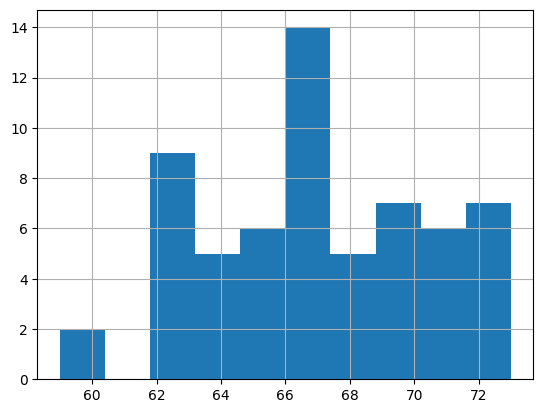
Patients in our data have a mean age of 61.8. The youngest and oldest patients are 21 and 91 years old, respectively. Recall from the documentation, all ages > 89 years old are capped at 91, so this is a nice sanity check that our maximum age is as expected.

Better yet, for a quick glance of the distribution, we can also use a histogram:

patients['anchor_age'].hist()

<Axes: >

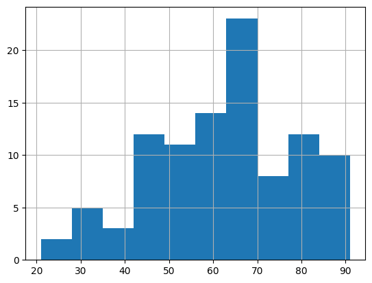
Checking the distribution of numerical values is important as it can help us quickly see if there is an unexpected observation in our data. For instance, perhaps we were told our dataset should only include adults, but we saw some ages that were < 10 years old. Or maybe someone is said to be 150 years old! These would necessitate further exploration to determine whether there are any data entry issues. Perhaps a busy doctor mistyped the age or maybe age was confused with a different variable.

Incorporating more data!

As previously mentioned, MIMIC contains multiple tables worth of data. Next, let’s look at a second file: vitals.csv which contains vital sign measurements for patients.

vitals = pd.read_csv('../../data/mimic_vitals.csv')

Let’s repeat the previously described steps to help us get to know our new vitals DataFrame.

vitals.head()

	subject_id	chartdate	result_name	result_value
0	10011398	2146-12-01	Height (Inches)	63
1	10011398	2147-01-22	Weight (Lbs)	127
2	10011398	2146-12-01	Weight (Lbs)	135
3	10011398	2147-07-24	Weight (Lbs)	136
4	10011398	2147-03-26	Weight (Lbs)	136

Once again, we see that the subject_id column is present, in addition to three new columns named: chartdate, result_name, and result_value.

Let’s see if the number of unique subject_ids match the number of rows:

vitals['subject_id'].nunique() == len(vitals)

False

len(vitals)

2964

In this case, it appears that there are many more observations in the vitals DataFrame (note: this was also apparent just from looking at the first 5 rows: the same subject_id appears in each row!).

To get a better idea of what is going on here, we can examine the specific types of categories in the result_name column. When we do, we learn that this variable annotates vital sign measurements including weight, height, body mass index (BMI), and blood pressure.

Since this dataset represents hospitalized patients, it is reasonable that each patient may have each vital measured several times throughout their hospital stay.

We can can confirm this by using .groupby() on the subject_id and result_name columns to see how many unique results (result_value) each patient had.

vitals.groupby(['subject_id', 'result_name'])[['result_value']].count()

		result_value
subject_id	result_name
10000032	BMI (kg/m2)	8
	Blood Pressure	6
	Height (Inches)	2
	Weight (Lbs)	25
10001217	BMI (kg/m2)	1
...	...	...
10039997	Weight (Lbs)	5
10040025	BMI (kg/m2)	10
	Blood Pressure	1
	Height (Inches)	1
	Weight (Lbs)	10

268 rows × 1 columns

As we did before, let’s also check the data types:

vitals.dtypes

subject_id       int64
chartdate       object
result_name     object
result_value    object
dtype: object

First, we can convert subject_id to a string again

vitals['subject_id'] = vitals['subject_id'].astype('str')

Working with Dates

Next, we see that chartdate is an object. We can convert dates to a special datetime data type in Python. This specification will allow us to perform operations between dates (e.g., finding the number of days between two blood pressure measurements).

vitals['chartdate'] = pd.to_datetime(vitals['chartdate'])
print(vitals.dtypes)
vitals.head()

subject_id              object
chartdate       datetime64[ns]
result_name             object
result_value            object
dtype: object

	subject_id	chartdate	result_name	result_value
0	10011398	2146-12-01	Height (Inches)	63
1	10011398	2147-01-22	Weight (Lbs)	127
2	10011398	2146-12-01	Weight (Lbs)	135
3	10011398	2147-07-24	Weight (Lbs)	136
4	10011398	2147-03-26	Weight (Lbs)	136

Note

Important Note about Dates

chartdate is the date the vital sign was recorded. You’ll notice that these years are in the future. Data shifting was performed to add an additional measure of privacy (as you may recall from #pillar-2-data-privacy). To protect the sensitive data of patients, dates were shifted up randomly for each patient, but in a consistent way (consistent shifting meaning if two blood presure measurements were taken on two back-to-back days, the shifted dates might look like: 2067-01-01 and 2067-01-02). Knowing whether or not a dataset’s dates are accurate or have been shifted is crucial if you’re trying to draw conclusions that are based on the actual date. For example, let’s say a patient was admitted with an unknown but severe respiratory infection in 1990, but had their dates shifted to 2020 - it would be completely erroneous to conclude they may have had COVID-19 (considering COVID-19 did not even exist in the 1990s!).

Now that chartdate has been converted to a datetime object, we can perform date-specific types of operations.

For instance, for each patient, let’s order rows in chronological order.

vitals_sorted = vitals.sort_values(by=['subject_id', 'chartdate'], ascending=[True, True])
vitals_sorted.head(10)

	subject_id	chartdate	result_name	result_value
1204	10000032	2180-04-27	Weight (Lbs)	94
1241	10000032	2180-04-27	Blood Pressure	110/65
1203	10000032	2180-05-07	Height (Inches)	60
1207	10000032	2180-05-07	BMI (kg/m2)	18.0
1218	10000032	2180-05-07	Weight (Lbs)	92.15
1219	10000032	2180-05-07	Weight (Lbs)	92.15
1220	10000032	2180-05-07	Weight (Lbs)	92.15
1221	10000032	2180-05-07	Weight (Lbs)	92.15
1222	10000032	2180-05-07	Weight (Lbs)	92.15
1223	10000032	2180-05-07	Weight (Lbs)	92.15

We can also calculate the difference in dates between a patient’s earliest measurement and most recent measurement. We can do this by first aggregating the min and max days using .agg() method and then calculating the difference in the number of days between the max and min dates by using Pandas .dt.days attribute.

date_range = vitals_sorted.groupby('subject_id')['chartdate'].agg(['min', 'max'])
date_range['day_diff'] = (date_range['max'] - date_range['min']).dt.days
date_range.sort_values('day_diff', ascending = True)

	min	max	day_diff
subject_id
10009049	2174-07-20	2174-07-20	0
10009628	2153-10-21	2153-10-21	0
10007818	2146-06-10	2146-06-10	0
10010471	2155-05-08	2155-05-08	0
10008454	2110-12-29	2110-12-29	0
...	...	...	...
10020306	2128-11-28	2135-08-20	2456
10004457	2141-10-30	2149-01-19	2638
10019003	2148-08-25	2155-11-23	2646
10015860	2186-10-14	2194-03-29	2723
10037928	2175-03-16	2183-12-25	3206

79 rows × 3 columns

Just from this sample we can see that some patients have years between measurements. This is reasonable since patients in MIMIC can be hospitalized more than once.

Other ways we could work with the datetime objects are by separating out the year, month, and day.

For example, if we wanted to create unique columns for year, month, and day, we could do the following:

vitals_sorted['year'] = vitals_sorted['chartdate'].dt.year
vitals_sorted['month'] = vitals_sorted['chartdate'].dt.month
vitals_sorted['day'] = vitals_sorted['chartdate'].dt.day

vitals_sorted

	subject_id	chartdate	result_name	result_value	year	month	day
1204	10000032	2180-04-27	Weight (Lbs)	94	2180	4	27
1241	10000032	2180-04-27	Blood Pressure	110/65	2180	4	27
1203	10000032	2180-05-07	Height (Inches)	60	2180	5	7
1207	10000032	2180-05-07	BMI (kg/m2)	18.0	2180	5	7
1218	10000032	2180-05-07	Weight (Lbs)	92.15	2180	5	7
...	...	...	...	...	...	...	...
2689	10040025	2147-12-29	Weight (Lbs)	212	2147	12	29
2696	10040025	2147-12-29	BMI (kg/m2)	34.2	2147	12	29
2692	10040025	2147-12-30	BMI (kg/m2)	30.3	2147	12	30
2704	10040025	2147-12-30	Weight (Lbs)	187.61	2147	12	30
2703	10040025	2148-01-19	Blood Pressure	112/60	2148	1	19

2964 rows × 7 columns

Data Wrangling Strings to Numbers

You may have noticed that result_name was not being recognized as a numerical variable. Perhaps there are non-numeric values in this column? We can check this using the following expression to see which observations have non-numeric characters:

# return the rows where there are non-numeric characters in `result_value`
vitals[vitals['result_value'].astype(str).str.contains(r'[^0-9]')][['result_name', 'result_value']].drop_duplicates()

	result_name	result_value
8	BMI (kg/m2)	23.6
9	BMI (kg/m2)	23.9
10	BMI (kg/m2)	25.3
12	BMI (kg/m2)	25.8
13	Height (Inches)	61.5
...	...	...
2957	Blood Pressure	152/94
2958	Blood Pressure	153/94
2961	Blood Pressure	111/72
2962	Blood Pressure	135/76
2963	Weight (Lbs)	252.65

1282 rows × 2 columns

You’ll notice in some cases that when result_name == Blood Pressure, the results contain a ‘/’ to separate systolic from diastolic blood pressure.

If we were interested in investigating blood pressure of these patients, we’d need to be mindful that Python will not allow us to simply average blood pressure without doing further data wrangling to separate these numbers from the non-numerical character.

# create blood pressure dataframe
bp_measurements = vitals.copy()

bp_measurements = bp_measurements[bp_measurements['result_name'] == 'Blood Pressure']
bp_measurements.head()

	subject_id	chartdate	result_name	result_value
14	10011398	2146-12-01	Blood Pressure	110/70
15	10011398	2147-03-26	Blood Pressure	112/80
16	10011398	2146-06-02	Blood Pressure	128/84
17	10011398	2147-07-24	Blood Pressure	132/84
18	10011398	2146-05-28	Blood Pressure	138/90

In the code below, we can use str.split() to help us separate systolic (number before /) and diastolic (number after /) blood pressure. Once we remove the /, we can also convert our new columns to integers.

bp_measurements[['systolic', 'diastolic']] = bp_measurements['result_value'].str.split('/', expand=True).astype(int)
print(bp_measurements.dtypes)
bp_measurements.head()

subject_id              object
chartdate       datetime64[ns]
result_name             object
result_value            object
systolic                 int64
diastolic                int64
dtype: object

	subject_id	chartdate	result_name	result_value	systolic	diastolic
14	10011398	2146-12-01	Blood Pressure	110/70	110	70
15	10011398	2147-03-26	Blood Pressure	112/80	112	80
16	10011398	2146-06-02	Blood Pressure	128/84	128	84
17	10011398	2147-07-24	Blood Pressure	132/84	132	84
18	10011398	2146-05-28	Blood Pressure	138/90	138	90

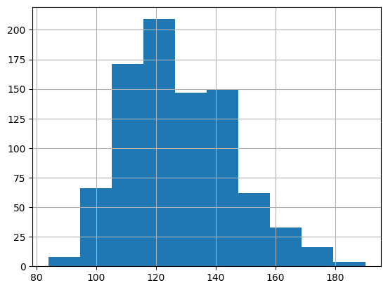
Examine distribution of continous variables

Let’s explore the distribution of our now cleaned systolic and diastolic variables

bp_measurements['systolic'].hist()

<Axes: >

bp_measurements['diastolic'].hist()

<Axes: >

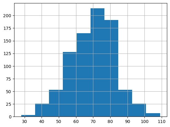
From these distributions, there does not appear to be any extreme outliers. However, if our primary analysis was to focus on blood pressure, we would likely want to consult a medical domain expert to ensure this distribution seems reasonable. Importantly, we would want to consider whether the the systolic and diastolic blood pressure values we see at either end of the distributions are biologically plausible.

Note

We refer to domain experts as those who have specialized knowledge in a field (i.e. domain) of interest. For example, domain experts might include medical doctors, physicists, CEOS, lawyers, etc. Often, domain experts might not know how to code or analyze data. However, domain experts can help clarify how the data was collected and what each variable means in the context of the particular domain. This can help ensure robust data wrangling.

Filtering Observations of Interest

Perhaps we are only interested in subjects who have height and weight measurements. We can create a new copy of the vitals dataframe and filter it to keep those observations of interest.

Note, from the result_name we see that height and weight are said to be recorded in inches and pounds (lbs), respectively.

height = vitals.copy()
height = height[height['result_name'] == 'Height (Inches)']

weight = vitals.copy()
weight = weight[weight['result_name'] == 'Weight (Lbs)']

Evaluate height

height.head()

	subject_id	chartdate	result_name	result_value
0	10011398	2146-12-01	Height (Inches)	63
13	10011398	2147-01-22	Height (Inches)	61.5
20	10014729	2125-02-22	Height (Inches)	65
21	10014729	2125-04-05	Height (Inches)	66
22	10014729	2126-01-24	Height (Inches)	66

First, let’s make sure that Python recognizes height as a continuous variable. If it’s not, we will convert it to type numeric.

# check variable data types
height.dtypes

subject_id              object
chartdate       datetime64[ns]
result_name             object
result_value            object
dtype: object

height['result_value'] = pd.to_numeric(height['result_value'])

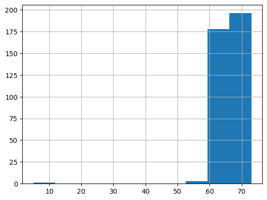
Identify the presence of outliers

As mentioned in an earlier chapter, outliers refer to observations that appear abnormal. Outliers may arise due to data-entry errors or, in this case, mistakes made during the actual vital sign measurements. It’s important to identify and investigate outliers so as to decide how we should handle them (if at all).

Visualing the distribution of a continous variable can help identify whether there are potential outliers. We can also use Pandas .describe() method to quickly calculate summary statistics.

height['result_value'].hist()

<Axes: >

# use describe() to compute summary statistics of the distribution
height['result_value'].describe()

count    378.000000
mean      67.105952
std        5.117295
min        5.000000
25%       63.500000
50%       67.000000
75%       71.000000
max       73.000000
Name: result_value, dtype: float64

Potential red flag: Is there really a patient who might be 5 inches tall? This is clearly a case we should investigate more.

First, we can sort the height values from lowest to highest in order to retrieve the subject_id of the patient who is said to have a height of 5 inches.

Sorting will also help us see whether there are any other patients with unusually low heights

height.sort_values(['result_value']).head()

	subject_id	chartdate	result_name	result_value
1844	10012853	2175-04-05	Height (Inches)	5.0
2883	10002428	2154-10-18	Height (Inches)	58.0
2885	10002428	2155-08-12	Height (Inches)	59.0
2884	10002428	2158-09-13	Height (Inches)	59.0
1203	10000032	2180-05-07	Height (Inches)	60.0

Let’s see if this patient has other recorded height measurements

height[height['subject_id']=='10012853']

	subject_id	chartdate	result_name	result_value
1844	10012853	2175-04-05	Height (Inches)	5.0
1845	10012853	2178-11-04	Height (Inches)	64.0
1846	10012853	2176-06-07	Height (Inches)	64.0
1847	10012853	2177-01-05	Height (Inches)	64.0

Interesting, it appears this patient had an initial obsevation of 5 inches, but then three years later was always measured at 64 inches (or 5’4 in feet/inches). It seems even further unlikely that a person would have that dramatic of a growth in such a short timespan. But, let’s investigate the variation in change for other patients who have more than one height measurement.

For each unique patient with multiple observations, we will calculate the standard deviation of each patient’s height measurements.

Note: ddof = 0 indicates that std for patients with one measurement will be displayed as 0 rather than NaN

import numpy as np

height['std'] = height.groupby('subject_id')['result_value'].transform('std', ddof=0)

height.sort_values('std', ascending = False)[['subject_id', 'std']].drop_duplicates().head(10)

	subject_id	std
1845	10012853	25.547749
1095	10005909	2.724312
461	10019917	1.000000
2720	10022880	0.942809
300	10001725	0.862706
0	10011398	0.750000
1265	10037928	0.745356
2729	10004457	0.731247
2884	10002428	0.707107
524	10005348	0.596212

It is obvious that our ‘concerning’ patient has a much higher standard deviation of their height measurements compared to other patients.

Let’s take a look at the two patients with the second and third highest standard deviation for comparison

height[height['subject_id']=='10005909']

	subject_id	chartdate	result_name	result_value	std
1094	10005909	2144-10-29	Height (Inches)	65.0	2.724312
1095	10005909	2144-12-10	Height (Inches)	70.0	2.724312
1096	10005909	2145-01-03	Height (Inches)	70.0	2.724312
1102	10005909	2144-11-15	Height (Inches)	72.5	2.724312

height[height['subject_id']=='10019917']

	subject_id	chartdate	result_name	result_value	std
461	10019917	2182-02-14	Height (Inches)	69.0	1.0
462	10019917	2182-01-09	Height (Inches)	71.0	1.0

It clearly seems that there the 5 inch observation is an outlier. Perhaps whoever recorded the data mistook the variable for feet instead of inches?

The best way to handle these types of inconsistencies will largely depend on the exact variable, research question of interest, and domain knowledge. In this case, it may be safe to take the median (64 years) for the concerning observation since this was a consistent height recorded over the following years. However, there are a couple of ways to best handle apparent outliers:

• Seek consultation from mentors and domain experts!

• Consider the age of the patient - height may be expected to change more dramatically over time for some patients rather than others. Depending on the patient’s age, it may be fair to take the next measurement that occured closest in time to the date of the suspect measurement.

Handling multiple observations

Despite the considerations metioned, let’s demonstrate how to groupby subject_id and take the median height for patients with multiple measurements.

# create a new variable with the median height value for each patient
height['result_value_median'] = height.groupby('subject_id')['result_value'].transform('median')

This next step ensures that we will now only have one unique row per patient.

# assuming we don't need to link by date
height_clean = height[['subject_id', 'result_name', 'result_value_median']].drop_duplicates()

# should have one observation per person
len(height_clean)

61

Let’s review the distribution again - now it looks a bit more normally distributed

height_clean['result_value_median'].hist()

<Axes: >

Unit Conversion Issues

Another important consideration when wrangling our data involves unit conversions. Errors involving unit conversions may show up as outliers.

Let’s next examine weight measurements.

### pre-process the data
weight['result_value'] = pd.to_numeric(weight['result_value'])

# calculate summary statistics
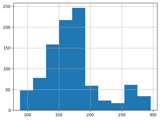
weight['result_value'].describe()

count    941.000000
mean     173.202763
std       44.009522
min       88.000000
25%      147.300000
50%      169.310000
75%      185.000000
max      296.000000
Name: result_value, dtype: float64

weight['result_value'].hist()

<Axes: >

Investigate the variance in measurements between patients with multiple observations

As we did with height, let’s calculate the standard deviation of weight measurements for patients with multiple weights recorded

weight['std'] = weight.groupby('subject_id')['result_value'].transform('std', ddof=0)# ddof = 0 indicates that std for patients with one measurement will be displayed as 0 rather than NaN

weight.sort_values('std', ascending = False)[['subject_id', 'std']].drop_duplicates().head(5)

	subject_id	std
177	10019385	58.385000
640	10021487	22.758934
1976	10019003	19.732249
1159	10039708	19.442869
2707	10040025	16.104849

Let’s examine the first patient who’s weight measurements have a std of 58.4.

When we look at this patient’s measurements, we may notice that they appear to have lost >110 pounds in < 1 month. Is this likely?

weight[weight['subject_id']=='10019385'].sort_values('chartdate')

	subject_id	chartdate	result_name	result_value	std
179	10019385	2180-02-15	Weight (Lbs)	214.07	58.385
177	10019385	2180-03-04	Weight (Lbs)	97.30	58.385

A unit conversion error may be a possibility here.

If we do the math, 1 pound ~ 0.45 kg.

If 214.07 is the weight in pounds, the equivalent weight in kilograms is 214.07*0.45 = ~96kg. These weight measurements made one month apart seem very close if we consider that there may be a unit conversion issue.

Let’s examine the second patient we observe having a high standard deviation as regards their weight measurements.

If we look at the measurements sorted chronologically, it looks like this second patient iteratively lost weight over the course of about 6 months before the weight began to increase again. This may be likely if the patient was sick and hospitalized for a long time and then began to recover and regain some of their weight.

weight[weight['subject_id']=='10021487'].sort_values('chartdate')

	subject_id	chartdate	result_name	result_value	std
644	10021487	2117-01-14	Weight (Lbs)	264.0	22.758934
643	10021487	2117-01-19	Weight (Lbs)	254.0	22.758934
641	10021487	2117-02-10	Weight (Lbs)	227.0	22.758934
638	10021487	2117-05-05	Weight (Lbs)	204.0	22.758934
635	10021487	2117-06-16	Weight (Lbs)	193.0	22.758934
656	10021487	2117-07-07	Weight (Lbs)	196.6	22.758934
636	10021487	2117-08-18	Weight (Lbs)	199.0	22.758934
637	10021487	2117-08-18	Weight (Lbs)	199.0	22.758934
639	10021487	2117-09-09	Weight (Lbs)	208.0	22.758934
657	10021487	2117-12-03	Weight (Lbs)	210.1	22.758934
640	10021487	2118-01-24	Weight (Lbs)	212.0	22.758934
642	10021487	2118-08-01	Weight (Lbs)	241.0	22.758934

While it may seem tedious, it is good practice to get in the habit of really getting to know your data. When specific observations jump out as being suspicious, you can perform case studies focused on particular patients to have a better sense of their data. In the case of the patient with rapid weight loss and regain, it may be helpful to referenmce additional data tables to have a more holistic view of this patient’s time in the hospital.

Non-standardized labels

Next, we will use a third MIMIC table: labs.csv to demonstrate measurements that have slightly different label names.

In this modified labs data, we have different types of hemoglobin and heparin laboratory (blood test) measurements (as noted in the label column).

labs = pd.read_csv('../../data/mimic_labs.csv')
labs.head()

	subject_id	label	value	valueuom
0	10000032	Hemoglobin	11.9	g/dL
1	10000032	MCHC	34.5	%
2	10001217	Hemoglobin	11.8	g/dL
3	10001217	MCHC	34.4	%
4	10001217	MCHC	32.4	%

Let’s take a look at the number of unique ways these labs may be represented. If we are not domain experts, we might not know whether there are differences in these blood tests.

For instance, if we are interested in examining hemoglobin levels, we could search the labs DataFrame for the string hemoglobin. When we do so, we’ll notice that there are many different variations of labs with “hemoglobin” in the name. Are all these the same? Sometimes the units (valueuom) can help us determine this. Othertimes, we may need to compare distributions or consult domain experts as to which are the proper variables to include.

labs[labs['label'].str.contains('hemoglobin', case = False)][['label', 'valueuom']].value_counts()

label              valueuom
Hemoglobin         g/dL        159
% Hemoglobin A1c   %            49
Carboxyhemoglobin  %             7
Methemoglobin      %             6
Hemoglobin C       %             1
Name: count, dtype: int64

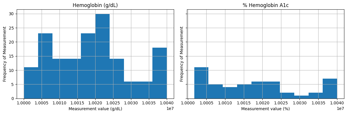
Let’s compare the distributions of the measurements labeled Hemoglobin (measured in g/dL) and % Hemoglobin A1c. Although the units different, the distributions seem fairly similar. This may warrent clinical domain expertise to review and confirm whether these lab measurements can combined.

import matplotlib.pyplot as plt

fig, axes = plt.subplots(1, 2, figsize=(12, 4), sharey=True)

labs[labs['label'] == 'Hemoglobin'].hist(ax=axes[0])
axes[0].set_title('Hemoglobin (g/dL)')
axes[0].set_ylabel('Frequency of Measurement')
axes[0].set_xlabel('Measurement value (g/dL)')

labs[labs['label'] == '% Hemoglobin A1c'].hist(ax=axes[1])
axes[1].set_title('% Hemoglobin A1c')
axes[1].set_ylabel('Frequency of Measurement')
axes[1].set_xlabel('Measurement value (%)')

plt.tight_layout()
plt.show()

Missing Data

Data wrangling is also necessary in the case of missing data.

There are many reasons for that data may be missing, and a full review of these is out of the scope of this textbook. However, common reasons for missing data include:

• Data entry problems

• Measurement was not recorded due to negligence or perhaps there is a reason the measurement wasn’t needed

Some common ways to handle missing data:

• Remove those measurements

• Impute the missing value using the mean or median

• Forward/backward filling

Rule of thumb: Talk to your domain experts/collaborators!

Let’s examine a simple, one patient case, for how we might work with missing blood pressure measurements. The following patient has multiple blood pressure measurements recorded.

bp_test = bp_measurements[bp_measurements['subject_id']=='10035631'][['chartdate', 'systolic']].sort_values('chartdate')

Let’s focus on a few time points when the patient had multiple measurements taken sequentially except for one day (2116-02-23).

bp_test = bp_test[(bp_test['chartdate'] >= '2116-02-16') & (bp_test['chartdate'] <='2116-02-24')]
bp_test

	chartdate	systolic
1826	2116-02-16	125
1760	2116-02-17	106
1777	2116-02-18	110
1796	2116-02-19	115
1748	2116-02-20	103
1785	2116-02-21	111
1799	2116-02-22	116
1753	2116-02-24	104

How might we handle missing values in this case?

One common way to handle missing values is to impute the missing value. Imputation refers to the process of filling in missing values. A simple method of imputation might include using the mean or the median value of a series of measurements in place of the missing value.

In this case, let’s demonstrate how we might use median imputation to replace the missing value.

First, in this case, we can see that there is not a row for 2116-02-23. Let’s use date_range() to create a complete series of dates. We can then re-index the original data so that we have a series of sequential dates.

full_range = pd.date_range(
    start='2116-02-16',
    end='2116-02-24',
    freq='D'
)
full_range

DatetimeIndex(['2116-02-16', '2116-02-17', '2116-02-18', '2116-02-19',
               '2116-02-20', '2116-02-21', '2116-02-22', '2116-02-23',
               '2116-02-24'],
              dtype='datetime64[ns]', freq='D')

# Reindex 
bp_test = (
    bp_test
    .set_index('chartdate')
    .reindex(full_range)
)

bp_test

	systolic
2116-02-16	125.0
2116-02-17	106.0
2116-02-18	110.0
2116-02-19	115.0
2116-02-20	103.0
2116-02-21	111.0
2116-02-22	116.0
2116-02-23	NaN
2116-02-24	104.0

After re-indexing, we have a complete set of dates. You will notice that there is a NaN next to the date that was originally missing a measurement. Next, we can use fillna() to replace the missing value by the median of the entire series.

# Impute the missing value with the median
bp_test_median = bp_test.fillna(bp_test.median())

# reset index to add `chartdate` as its own column
bp_test_median = bp_test_median.reset_index().rename(columns={'index': 'chartdate'})

bp_test_median

	chartdate	systolic
0	2116-02-16	125.0
1	2116-02-17	106.0
2	2116-02-18	110.0
3	2116-02-19	115.0
4	2116-02-20	103.0
5	2116-02-21	111.0
6	2116-02-22	116.0
7	2116-02-23	110.5
8	2116-02-24	104.0

We could also impute by forward filling, which is an imputation technique referring to when the last observation is carried forward to replace a missing value.

# Impute the missing value with the median
bp_test_forward = bp_test.ffill()

# reset index to add `chartdate` as its own column
bp_test_forward = bp_test_forward.reset_index().rename(columns={'index': 'chartdate'})

bp_test_forward

	chartdate	systolic
0	2116-02-16	125.0
1	2116-02-17	106.0
2	2116-02-18	110.0
3	2116-02-19	115.0
4	2116-02-20	103.0
5	2116-02-21	111.0
6	2116-02-22	116.0
7	2116-02-23	116.0
8	2116-02-24	104.0

Warning

It’s always important to think critically about the best ways to impute any missing data. We demonstrated two simple methods (median/mean imputation and forward filling), but there are entire books written on different imputation techniques. As mentioned throughout this chapter, discussions with your collaboraters and domain experts are important for identifying the best imputation method.

If imputation is used, it’s important to be careful that methods we used are not biased. For example, mean imputation may not be preferred if the data is highly skewed.

Another imputation method called backward filling refers to when a missing value is replaced by carrying the next observation backwards. As you can imagine, this can be problematic in cases when we are trying to time series data to predict some future outcome. We may be making our task much easier owing to data leakage, as you learned in the chapter on feature engineering.

Conclusions

This chapter aimed to provide you with a real-world dataset that benefited from data wrangling. As you can see, the process of data wrangling is highly dependent on your dataset. In many cases, there is also not one correct way to go about these processes. What’s important is to deeply consider what our data represents, how it’s structured, and the downstream implications for our analysis if we do or do not prepare our data appropriately. Data wrangling is also a great opportunity to work deeply with your collaborators (domain experts!) to ensure each step of the process is grounded in practical utility and is reflective of how the data was generated, collected, and how it’s meant to be analyzed.

[^*] Johnson, A., Bulgarelli, L., Pollard, T., Gow, B., Moody, B., Horng, S., Celi, L. A., & Mark, R. (2024). MIMIC-IV (version 3.1). PhysioNet. RRID:SCR_007345. https://doi.org/10.13026/kpb9-mt58

[^**] Johnson, A., Bulgarelli, L., Pollard, T., Horng, S., Celi, L. A., & Mark, R. (2023). MIMIC-IV Clinical Database Demo (version 2.2). PhysioNet. RRID:SCR_007345. https://doi.org/10.13026/dp1f-ex47