
24.4. Training a Neural Network#
Now that we understand how neural networks are structured, we need to understand how they learn from data. The weights and biases are the key parameters of a neural network. By adjusting these parameters, the model learns how to weigh different input features and make accurate predictions. But how do we find the right values for these parameters?
The first thing we need is a dataset to learn from—the training dataset. Our goal is to find an algorithm that helps us determine weights and biases so that the predicted output from the network \(\hat{y}(x)\) is a good approximation of \(y(x)\) (the true output) for all training inputs \(x\). To quantify how well we are achieving this goal, we define a loss function (also called a cost function). The loss function measures the difference between our network’s predictions and the true values—the smaller the loss, the better our network is performing.
Different problems require different loss functions. Some common examples include averaging the following quantities over all training samples:
Mean Squared Error (regression): \((y-\hat{y})^2\)
Mean Absolute Error (regression): \(|y-\hat{y}|\)
Binary Cross-Entropy (binary classification, where \(y \in \{0,1\}\) and \(\hat{y}\) is the predicted probability): \(-[y\log \hat{y}+(1-y)\log (1-\hat{y})]\)
Categorical Cross-Entropy (multi-class classification with \(c\) classes): \(-\sum_{i=1}^{c} y_i \cdot \log \hat{y}_i\)
The prediction \(\hat{y}\) made by the model is a function of the input features and all the network parameters (weights and biases throughout all layers). The aim of our training algorithm is to find the values of weights and biases that make the loss function as small as possible.
One way to minimize a function is to do it analytically using calculus. We take the derivative of the function with respect to each variable (the partial derivatives), set them equal to zero to find critical points, and use higher-order derivatives to determine whether these points are minima. Neural networks, however, have an enormous number of parameters (often in millions or even billions). Because the loss function depend on these billions of parameters in a very complicated way, solving for minimum analytically becomes computationally prohibitive!
Instead, we use an algorithm called gradient descent to perform this minimization.
Gradient Descent#
To understand gradient descent, we are going to temporarily forget about the specific form of our loss function and instead focus on understanding how the algorithm works for minimizing any general function \(f\) of many variables.
Consider the following analogy. Suppose you are standing in a valley and trying to reach the lowest point. Instead of trying to view the entire valley at once to find the minimum point, you simply look around from where you are to find the direction where the slope descends most steeply. You then take a small step in that direction. From this new position, you again look for the direction of steepest descent and take another small step. You continue this process, with the goal of reaching the bottom through a series of steps. As long as each step goes downhill, you will eventually reach the bottom (or at least a low point, called local minima in math language).
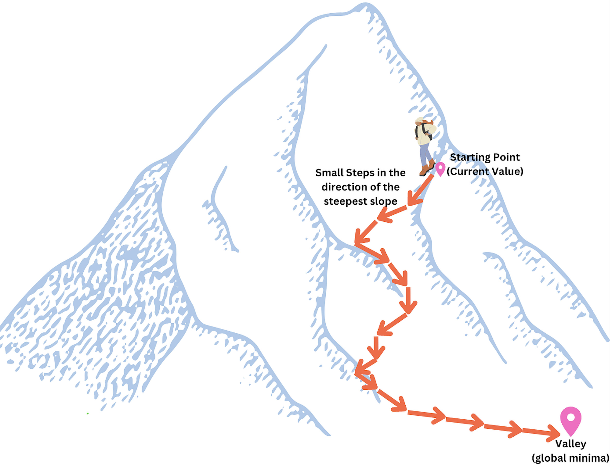
Figure: Gradient Descent Analogy Image Source
To make this more precise, let us say we have a function \(f\) of two variables \(x_1\) and \(x_2\). If we move a small amount \(\Delta x_1\) in the direction of \(x_1\) and \(\Delta x_2\) in the direction of \(x_2\), then calculus tells us that our function will change approximately as follows:
We need to calculate this quantity at our current point to determine how much our function will change when we move from that point.
Our goal is to find a way of choosing \(\Delta x_1\) and \(\Delta x_2\) so that \(\Delta f\) is negative—meaning we are reducing our function value, or in other words, moving toward the minimum.
We can rewrite the equation for \(\Delta f\) more compactly as:
where \(\nabla f = \left( \frac{\partial f}{\partial x_1}, \frac{\partial f}{\partial x_2} \right)\) and \(\Delta x = \left( \Delta x_1, \Delta x_2 \right)\). The dot in this formula represents the dot product of vectors.
The vector \(\nabla f\) relates the changes in \(x\) to changes in \(f\) and is known as the gradient of \(f\). The word “gradient” literally means inclination and refers to an increase or decrease in the magnitude of a property observed when passing from one point to another. We see that \(\nabla f\) is precisely measuring that. The vector \(\Delta x\) is simply a measure of how much we are moving and in what direction.
The gradient vector is known to point in the direction where the function increases most rapidly. So, if we want to decrease the function, we should move in the opposite direction of the gradient. Therefore, we choose:
where \(\eta\) is small, positive parameter (known as the learning rate). The change in \(f\) becomes \(\Delta f \approx -\eta \nabla f \cdot \nabla f = - \eta ||\nabla f||^2\). The term \(||\nabla f||^2\) is squared length of a vector and is therefore always positive (or zero). This means, \(\Delta f \leq 0\) i.e. f decreases which such a choice of \(\Delta x\).
Here is how the algorithm works in practice. Suppose you start at a random point \((x_1^{(0)}, x_2^{(0)})\). You compute the gradient \(\nabla f\) at this point and take a step to reach the new point:
Once you are at this new point, you repeat the process: compute the gradient at \((x_1^{(1)}, x_2^{(1)})\) and move to \((x_1^{(2)}, x_2^{(2)})\), and so on. With each step, you reduce the value of the function \(f\) until, we hope, you reach a minimum.
To make this algorithm work effectively, we need to choose the learning rate \(\eta\) carefully. If we choose \(\eta\) too large, we might take steps that are too big, potentially overshooting the minimum and even increasing the function value. On the other hand, if we choose \(\eta\) too small, the algorithm will take tiny steps and run very slowly, requiring many iterations to reach the minimum.
Gradient descent does have some limitations. Firstly, it depends on a good choice of learning rate. Additionally, we typically start at a random point in the space, and that starting point may not be ideal. The algorithm is guaranteed to find a local minimum (a nearby dip in the landscape), but not necessarily the global minimum (the absolute lowest point). Despite these limitations, gradient descent works well in practice as an optimization algorithm.
When we have large datasets, computing the gradient using all training examples at once can be very slow. Stochastic gradient descent (SGD) speeds up the process by using only a small random subset of the data, called a mini-batch, to estimate the gradient at each step. In practice, most neural networks are trained using SGD or its variants (such as momentum, RMSProp, or Adam).
Note
Understanding how neural networks are trained is important for developing conceptual insight into how these models learn. However, in practice, modern software libraries such as TensorFlow and PyTorch handle the training process in a largely automated way. These tools compute gradients, update parameters, and manage the optimization steps for us, allowing users to train complex neural networks without manually implementing the underlying mathematical procedures.
Chapter References: