Implementing Ensemble Methods with Python

25.5. Implementing Ensemble Methods with Python#

In this section, we will see how to implement the ensemble methods we learned in the previous section using Python. We will work with the Titanic dataset, which contains information about passengers and whether they survived.

Earlier in the chapter, we preprocessed the data by handling missing values and encoding categorical variables. We work with the same preprocessed dataset. If you click on the following code cell shows, it will show you the pre processing we performed.

	Survived	Pclass	Age	SibSp	Parch	Fare	Sex	Embarked
0	0	3	22.0	1	0	7.2500	1	2
1	1	1	38.0	1	0	71.2833	0	0
2	1	3	26.0	0	0	7.9250	0	2
3	1	1	35.0	1	0	53.1000	0	2
4	0	3	35.0	0	0	8.0500	1	2
...	...	...	...	...	...	...	...	...
885	0	3	39.0	0	5	29.1250	0	1
886	0	2	27.0	0	0	13.0000	1	2
887	1	1	19.0	0	0	30.0000	0	2
889	1	1	26.0	0	0	30.0000	1	0
890	0	3	32.0	0	0	7.7500	1	1

712 rows × 8 columns

Before building our ensemble models, we need to split the data into training and test sets. We make this split using the train_test_split function from scikit-learn’s model_selection module.

from sklearn.model_selection import train_test_split

X = Titanic_df.drop(columns=['Survived'])
y = Titanic_df['Survived']
X_train, X_test, y_train, y_test = train_test_split(X, y, test_size=0.2, random_state=10)

The function takes our feature matrix X and target variable y, and returns four datasets: X_train and y_train for training, and X_test and y_test for testing. The test_size=0.2 parameter allocates 20% of the data for testing. The random_state=10 parameter ensures reproducibility by producing the same random split each time.

We will implement three ensemble methods: Bagging, Random Forests, and AdaBoost. We will train each method on the training data, evaluate their performance on the test data, and compare their results to see which performs best for predicting Titanic survival.

Bagging#

We can implement bagging in Python using scikit-learn’s BaggingClassifier. See here for documentation.

The parameters we use in creating our bagging model are:

estimator: The base model to use. Here, we use DecisionTreeClassifier() i.e. our building blocks are decision trees.
n_estimators: The number of bootstrap training datasets and trees to create. We use 100 trees.
random_state: Ensures we get the same results every time we run the code, making it reproducible.

from sklearn.ensemble import BaggingClassifier
from sklearn.tree import DecisionTreeClassifier

# Create a bagging classifier with decision trees as weak learners
bagging_model = BaggingClassifier(
    estimator=DecisionTreeClassifier(),
    n_estimators=100,
    random_state=42
)

# Train the model
bagging_model.fit(X_train, y_train)

BaggingClassifier(estimator=DecisionTreeClassifier(), n_estimators=100,
                  random_state=42)

In a Jupyter environment, please rerun this cell to show the HTML representation or trust the notebook.
On GitHub, the HTML representation is unable to render, please try loading this page with nbviewer.org.

Lets see how the 100 trees in our bagging ensemble vote for the first passenger in our test set.

# Get predictions from all trees for the first test example
tree_predictions = [tree.predict([X_test.iloc[0].values]) for tree in bagging_model.estimators_]
votes = np.array(tree_predictions).flatten()

print(f"Trees voting 'Survived': {np.sum(votes == 1)}")
print(f"Trees voting 'Not Survived': {np.sum(votes == 0)}")

Trees voting 'Survived': 33
Trees voting 'Not Survived': 67

Since we use majority vote in classification, we would therefore predict the first passenger to not survive. We now make the predictions on the whole test set and evaluate the model’s overall accuracy. For that, we import accuracy_score from sklearn.metrics.

# Make predictions
y_pred_bagging = bagging_model.predict(X_test)

from sklearn.metrics import accuracy_score

# Evaluate accuracy
bagging_accuracy = accuracy_score(y_test, y_pred_bagging)
print(f"Bagging Accuracy: {bagging_accuracy:.4f}")

Bagging Accuracy: 0.8042

This means our bagging model correctly predicts survival for approximately 80% of the passengers in the test set.

We can also visualize the feature importance for each of the features used in the modeling. Each tree calculates its own feature importance based on the bootstrap sample it was trained on. We average these importances across all trees to get a more robust estimate of which features are most important for prediction.

# Calculate average feature importance across all trees
importances = np.mean([tree.feature_importances_ for tree in bagging_model.estimators_], axis=0)

# Sort features by importance
indices = np.argsort(importances)
sorted_features = X_train.columns[indices]
sorted_importances = importances[indices]

# Plot
plt.barh(sorted_features, sorted_importances)
plt.xlabel('Importance')
plt.title('Feature Importances in Bagging')
plt.show()

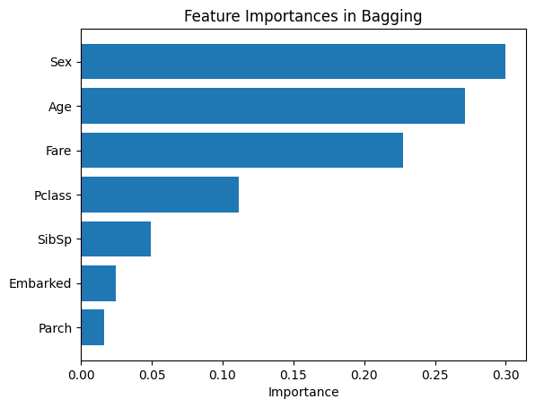
../../_images/7be173a26e34bcb6a74ad3796559f229db570c188084d8b4f0364a3389f9d388.png

From our bar chart, it looks like Sex, Age, and Fare played the most important role in predicting survival. Now, we do the same modeling with Random Forest and AdaBoost.

Random Forest#

We implement Random Forests using scikit-learn’s RandomForestClassifier. See here for documentation.

We set the following parameters:

n_estimators: The number of trees in the forest. We use 100 trees, same as in bagging.
random_state: To ensures reproducibility.

By default, RandomForestClassifier uses \(m = \sqrt{p}\) features at each split for classification, where \(p\) is the total number of features. With our 7 features, \(\sqrt{7} \approx 2.65\), so 2 features are randomly selected at each split.

from sklearn.ensemble import RandomForestClassifier

# Create a Random Forest classifier
rf_model = RandomForestClassifier(
    n_estimators=100,
    random_state=42
)

# Train the model
rf_model.fit(X_train, y_train)

# Make predictions
y_pred_rf = rf_model.predict(X_test)

# Evaluate accuracy
rf_accuracy = accuracy_score(y_test, y_pred_rf)
print(f"Random Forest Accuracy: {rf_accuracy:.4f}")

Random Forest Accuracy: 0.8112

Our Random Forest model achieves approximately 81% accuracy, which is a slight improvement over the Bagging model (80%). This demonstrates how the additional randomness of feature selection can lead to better predictions. Lets compare the importance of the features in random forest model with bagging.

# Get feature importances and sort features by importance
rf_importances = rf_model.feature_importances_
indices = np.argsort(rf_importances)  
sorted_features = X_train.columns[indices]
sorted_importances = rf_importances[indices]

# Plot (barh displays bottom to top, so ascending = highest at top)
plt.barh(sorted_features, sorted_importances)
plt.xlabel('Importance')
plt.title('Feature Importances in Random Forest')
plt.show()

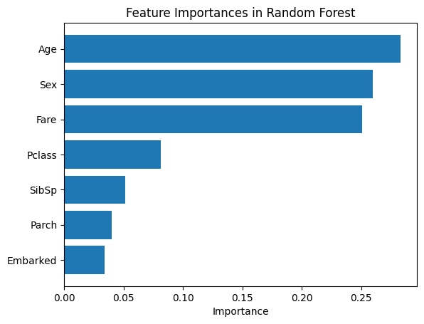
../../_images/1a83205c1203314fa017ce1a44a950f728a962c4c3fdabba2c65656f761fe4cc.png

Similar to Bagging, Sex, Age, and Fare remain the most important features. However, Random Forest ranks Age higher than Sex, showing how random feature selection can shift feature importance rankings.

AdaBoost#

We implement AdaBoost using scikit-learn’s AdaBoostClassifier. See here for documentation.

We set the following parameters:

estimator: The base model to use. We use DecisionTreeClassifier(max_depth=1) to create stumps (trees with only one split).
n_estimators: The number of boosting iterations (stumps to create). We use 100.
random_state: Ensures reproducibility.

from sklearn.ensemble import AdaBoostClassifier

# Create an AdaBoost classifier
adaboost_model = AdaBoostClassifier(
    estimator=DecisionTreeClassifier(max_depth=1),
    n_estimators=100,
    random_state=42
)

# Train the model
adaboost_model.fit(X_train, y_train)

# Make predictions
y_pred_adaboost = adaboost_model.predict(X_test)

# Evaluate accuracy
adaboost_accuracy = accuracy_score(y_test, y_pred_adaboost)
print(f"AdaBoost Accuracy: {adaboost_accuracy:.4f}")

AdaBoost Accuracy: 0.7832

For our dataset, AdaBoost shows the best prediction accuracy so far of 82.52%. Let us visualize the feature importance in this case.

# Get feature importances and sort features by importance
adaboost_importances = adaboost_model.feature_importances_
indices = np.argsort(adaboost_importances)
sorted_features = X_train.columns[indices]
sorted_importances = adaboost_importances[indices]

# Plot
plt.barh(sorted_features, sorted_importances)
plt.xlabel('Importance')
plt.title('Feature Importances in AdaBoost')
plt.show()

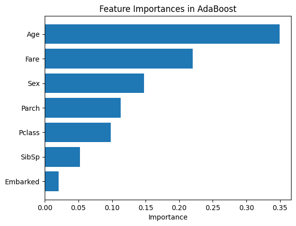
../../_images/937f930a53b43b057562db23d128e3b0329a6afff03d3f76164f0d00ca0b450a.png

The feature importance pattern in AdaBoost differs significantly from the other methods. Fare is by far the most important feature, with Age being moderately important followed by SibSp. All other features, including Sex which was highly important in Bagging and Random Forests, show much lower importance in AdaBoost.

This shows an important characteristic of AdaBoost with stumps: since each stump makes only a single split, the sequential learning process can emphasize different features than methods using deeper trees. This is not an error, but rather reflects how different ensemble approaches can prioritize features differently even on the same data.

Hyperparameter Tuning with Grid Search#

So far, we have manually selected hyperparameters for our models. For example, in Random Forest, we chose n_estimators=100 and used the default value for max_features (which is ‘sqrt’). While these are reasonable choices, they may not be optimal. Selecting the right hyperparameters is crucial for achieving the best model performance, but manually testing different combinations can be time-consuming and inefficient.

Grid search is a systematic method for hyperparameter tuning that automates this process. It evaluates a predefined set of hyperparameter combinations to find the configuration that produces the best performance.

Think of grid search as exploring a grid where each axis represents a hyperparameter, and each point on the grid represents a specific combination of hyperparameter values. Grid search exhaustively tests each combination to find the best one.

Grid search involves three main components:

Hyperparameter Space: The range of values to explore for each hyperparameter. For example, testing n_estimators values of 50, 100, and 200.
Scoring Metric: The performance metric used to evaluate each combination, such as accuracy or F1-score.
Cross-Validation: Recall that cross-validation splits the training data into multiple folds to evaluate performance more reliably, ensuring the results are not due to a particular split of the data.

Let us apply grid search to tune our Random Forest model. Note that Random Forest has many hyperparameters, and we have been using their default values so far. Here, we will tune four key hyperparameters:

n_estimators: The number of trees in the forest.
max_depth: The maximum depth of each tree.
max_features: The number of features to consider when looking for the best split. Recall that the default for classification is 'sqrt'.
min_samples_split: The minimum number of samples required to split an internal node.

Please see the documentation for more hyperparameters and their default values.

# Import necessary libraries
from sklearn.model_selection import GridSearchCV

# Create a Random Forest Classifier
random_forest_model = RandomForestClassifier(random_state=42)

# Define the parameter grid for grid search
param_grid = {
    'n_estimators': [50, 100, 150, 200],
    'max_depth': [None, 20, 30],  # Include None
    'max_features': ['sqrt', 'log2', None],
    'min_samples_split': [2, 5, 10]
}

# Perform grid search with cross-validation
grid_search = GridSearchCV(random_forest_model, param_grid, cv=10, scoring='accuracy')
grid_search.fit(X_train, y_train)

# Get the best parameters from grid search
best_params = grid_search.best_params_
print(f"Best Parameters: {best_params}")

# Get the best model 
best_random_forest_model = grid_search.best_estimator_

# Make predictions on the test data
predictions = best_random_forest_model.predict(X_test)

# Evaluate the model accuracy
accuracy = accuracy_score(y_test, predictions)
print(f"Random Forest Accuracy with Grid Search: {accuracy:.4f}")

Best Parameters: {'max_depth': None, 'max_features': 'sqrt', 'min_samples_split': 10, 'n_estimators': 50}
Random Forest Accuracy with Grid Search: 0.8112

In the above grid search, we tested \(4 \times 3 \times 3 \times 3 = 108\) different combinations of hyperparameter values using cross-validation.

Grid search identified the best combination as: unlimited tree depth (max_depth=None), square root of features at each split (max_features='sqrt'), minimum of 10 samples required to split a node (min_samples_split=10), and 50 trees in the forest (n_estimators=50). This configuration achieves an accuracy of 81.12% which is the same as our original Random Forest model. However, there is an important advantage: the tuned model uses only 50 trees instead of 100, meaning it trains approximately twice as fast while maintaining the same predictive performance. This illustrates how hyperparameter tuning can find more efficient configurations without sacrificing performance.

New in This Chapter

	estimator estimator: object, default=None The base estimator to fit on random subsets of the dataset. If None, then the base estimator is a :class:`~sklearn.tree.DecisionTreeClassifier`. .. versionadded:: 1.2 `base_estimator` was renamed to `estimator`.	DecisionTreeClassifier()
	n_estimators n_estimators: int, default=10 The number of base estimators in the ensemble.	100
	max_samples max_samples: int or float, default=None The number of samples to draw from X to train each base estimator (with replacement by default, see `bootstrap` for more details). - If None, then draw `X.shape[0]` samples irrespective of `sample_weight`. - If int, then draw `max_samples` samples. - If float, then draw `max_samples * X.shape[0]` unweighted samples or `max_samples * sample_weight.sum()` weighted samples.	None
	max_features max_features: int or float, default=1.0 The number of features to draw from X to train each base estimator ( without replacement by default, see `bootstrap_features` for more details). - If int, then draw `max_features` features. - If float, then draw `max(1, int(max_features * n_features_in_))` features.	1.0
	bootstrap bootstrap: bool, default=True Whether samples are drawn with replacement. If False, sampling without replacement is performed. If fitting with `sample_weight`, it is strongly recommended to choose True, as only drawing with replacement will ensure the expected frequency semantics of `sample_weight`.	True
	bootstrap_features bootstrap_features: bool, default=False Whether features are drawn with replacement.	False
	oob_score oob_score: bool, default=False Whether to use out-of-bag samples to estimate the generalization error. Only available if bootstrap=True.	False
	warm_start warm_start: bool, default=False When set to True, reuse the solution of the previous call to fit and add more estimators to the ensemble, otherwise, just fit a whole new ensemble. See :term:`the Glossary `. .. versionadded:: 0.17 warm_start constructor parameter.	False
	n_jobs n_jobs: int, default=None The number of jobs to run in parallel for both :meth:`fit` and :meth:`predict`. ``None`` means 1 unless in a :obj:`joblib.parallel_backend` context. ``-1`` means using all processors. See :term:`Glossary ` for more details.	None
	random_state random_state: int, RandomState instance or None, default=None Controls the random resampling of the original dataset (sample wise and feature wise). If the base estimator accepts a `random_state` attribute, a different seed is generated for each instance in the ensemble. Pass an int for reproducible output across multiple function calls. See :term:`Glossary `.	42
	verbose verbose: int, default=0 Controls the verbosity when fitting and predicting.	0

	criterion criterion: {"gini", "entropy", "log_loss"}, default="gini" The function to measure the quality of a split. Supported criteria are "gini" for the Gini impurity and "log_loss" and "entropy" both for the Shannon information gain, see :ref:`tree_mathematical_formulation`.	'gini'
	splitter splitter: {"best", "random"}, default="best" The strategy used to choose the split at each node. Supported strategies are "best" to choose the best split and "random" to choose the best random split.	'best'
	max_depth max_depth: int, default=None The maximum depth of the tree. If None, then nodes are expanded until all leaves are pure or until all leaves contain less than min_samples_split samples.	None
	min_samples_split min_samples_split: int or float, default=2 The minimum number of samples required to split an internal node: - If int, then consider `min_samples_split` as the minimum number. - If float, then `min_samples_split` is a fraction and `ceil(min_samples_split * n_samples)` are the minimum number of samples for each split. .. versionchanged:: 0.18 Added float values for fractions.	2
	min_samples_leaf min_samples_leaf: int or float, default=1 The minimum number of samples required to be at a leaf node. A split point at any depth will only be considered if it leaves at least ``min_samples_leaf`` training samples in each of the left and right branches. This may have the effect of smoothing the model, especially in regression. - If int, then consider `min_samples_leaf` as the minimum number. - If float, then `min_samples_leaf` is a fraction and `ceil(min_samples_leaf * n_samples)` are the minimum number of samples for each node. .. versionchanged:: 0.18 Added float values for fractions.	1
	min_weight_fraction_leaf min_weight_fraction_leaf: float, default=0.0 The minimum weighted fraction of the sum total of weights (of all the input samples) required to be at a leaf node. Samples have equal weight when sample_weight is not provided.	0.0
	max_features max_features: int, float or {"sqrt", "log2"}, default=None The number of features to consider when looking for the best split: - If int, then consider `max_features` features at each split. - If float, then `max_features` is a fraction and `max(1, int(max_features * n_features_in_))` features are considered at each split. - If "sqrt", then `max_features=sqrt(n_features)`. - If "log2", then `max_features=log2(n_features)`. - If None, then `max_features=n_features`. .. note:: The search for a split does not stop until at least one valid partition of the node samples is found, even if it requires to effectively inspect more than ``max_features`` features.	None
	random_state random_state: int, RandomState instance or None, default=None Controls the randomness of the estimator. The features are always randomly permuted at each split, even if ``splitter`` is set to ``"best"``. When ``max_features < n_features``, the algorithm will select ``max_features`` at random at each split before finding the best split among them. But the best found split may vary across different runs, even if ``max_features=n_features``. That is the case, if the improvement of the criterion is identical for several splits and one split has to be selected at random. To obtain a deterministic behaviour during fitting, ``random_state`` has to be fixed to an integer. See :term:`Glossary ` for details.	None
	max_leaf_nodes max_leaf_nodes: int, default=None Grow a tree with ``max_leaf_nodes`` in best-first fashion. Best nodes are defined as relative reduction in impurity. If None then unlimited number of leaf nodes.	None
	min_impurity_decrease min_impurity_decrease: float, default=0.0 A node will be split if this split induces a decrease of the impurity greater than or equal to this value. The weighted impurity decrease equation is the following:: N_t / N * (impurity - N_t_R / N_t * right_impurity - N_t_L / N_t * left_impurity) where ``N`` is the total number of samples, ``N_t`` is the number of samples at the current node, ``N_t_L`` is the number of samples in the left child, and ``N_t_R`` is the number of samples in the right child. ``N``, ``N_t``, ``N_t_R`` and ``N_t_L`` all refer to the weighted sum, if ``sample_weight`` is passed. .. versionadded:: 0.19	0.0
	class_weight class_weight: dict, list of dict or "balanced", default=None Weights associated with classes in the form ``{class_label: weight}``. If None, all classes are supposed to have weight one. For multi-output problems, a list of dicts can be provided in the same order as the columns of y. Note that for multioutput (including multilabel) weights should be defined for each class of every column in its own dict. For example, for four-class multilabel classification weights should be [{0: 1, 1: 1}, {0: 1, 1: 5}, {0: 1, 1: 1}, {0: 1, 1: 1}] instead of [{1:1}, {2:5}, {3:1}, {4:1}]. The "balanced" mode uses the values of y to automatically adjust weights inversely proportional to class frequencies in the input data as ``n_samples / (n_classes * np.bincount(y))`` For multi-output, the weights of each column of y will be multiplied. Note that these weights will be multiplied with sample_weight (passed through the fit method) if sample_weight is specified.	None
	ccp_alpha ccp_alpha: non-negative float, default=0.0 Complexity parameter used for Minimal Cost-Complexity Pruning. The subtree with the largest cost complexity that is smaller than ``ccp_alpha`` will be chosen. By default, no pruning is performed. See :ref:`minimal_cost_complexity_pruning` for details. See :ref:`sphx_glr_auto_examples_tree_plot_cost_complexity_pruning.py` for an example of such pruning. .. versionadded:: 0.22	0.0
	monotonic_cst monotonic_cst: array-like of int of shape (n_features), default=None Indicates the monotonicity constraint to enforce on each feature. - 1: monotonic increase - 0: no constraint - -1: monotonic decrease If monotonic_cst is None, no constraints are applied. Monotonicity constraints are not supported for: - multiclass classifications (i.e. when `n_classes > 2`), - multioutput classifications (i.e. when `n_outputs_ > 1`), - classifications trained on data with missing values. The constraints hold over the probability of the positive class. Read more in the :ref:`User Guide `. .. versionadded:: 1.4	None

Implementing Ensemble Methods with Python

Contents

25.5. Implementing Ensemble Methods with Python#

Bagging#

Random Forest#

AdaBoost#

Hyperparameter Tuning with Grid Search#

Terms

Code