
19.1. Feature Engineering#
Datasets in machine learning can broadly be categorized as structured and unstructured, depending on its format of presentation:
Structured data: Structured data is typically stored in tabular formats with a well-defined schema that every single row or datapoint adheres to when being recorded. Structured data can include both quantitative measurements (prices, height, etc.) as well as qualitative records (dates, names, addresses, etc.) This kind of data works well with most machine learning algorithms, can be easy to maintain and interpret.
Example of structured data : Below is a dataset that we have previously used for data analysis. It contains information on different houses in Athens, Ohio. Every record indicates the relationship between the various features of a residence listed in this data and the price at which it was sold in the market. The data is structured because every record is represented using the same set of attributes.
Unstructured data: Unstructured data does not have a standard, pre-defined format and typically resembles data in its raw form as closely as possible. Data consisting of texts, images, videos or multimedia files typically fall under this category.
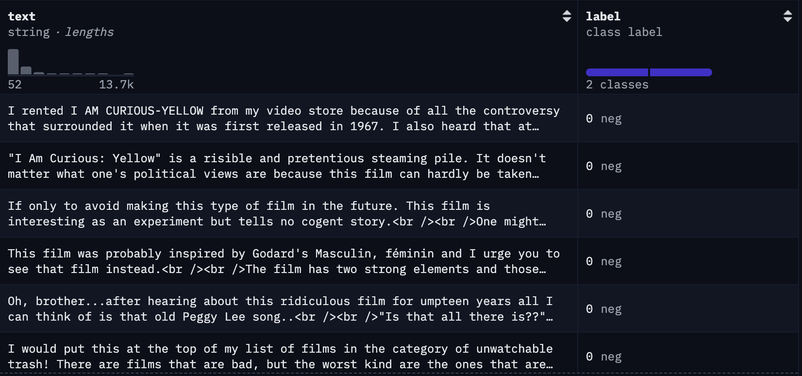
Example of unstructured data: Here is a snapshot of the popular IMDB dataset often used to train models that consume text snippets to predict the sentiment expressed in them. The dataset contains 50K reviews posted by users of the website with a positive or negative sentiment label. Unlike the housing data shown above, the input is not represented through a fixed set of features and instead the text itself is the only feature available.
Feature engineering strategies vary depending on the type and format of data to which they are being applied.
Features in Machine Learning#
Most machine learning tasks start with data retrieval that gathers raw data to be ingested into a model. This is followed by a data preparation process where different techniques are tried to engineer meaningful features that the model of choice can utilize during training. The trained model is then deployed for the subsequent prediction (regression or classification) task on unseen data. Note that data used for testing also undergo similar transformations, made earlier on the training data, prior to being fed to the model to generate predictions.
Feature Engineering Techniques in Structured Data#
Structured data is standardized, clearly defined in format, as well as easy to organize, search and analyze. As mentioned before, data types stored in structured data can be both numeric or categorical. We will look into specific feature engineering techniques for each of these data types now.
Feature Engineering on Numeric Data#
Numeric or quantitative data consist of scalar values that record measurements or observations, often in certain prespecified units. You can learn more about this type of data in Section 9.2.
Raw numeric data can be fed directly into most models but depending on the problem and application domain they could still be modified to better features. In this section, we will look into a few strategies we can leverage for feature engineering on numeric data. We will use two datasets at our disposal to demonstrate these techniques.
Let’s begin our review of feature engineering techniques by applying them on the previously used diabetes dataset.
The subjects of this dataset are pregnant people aged 21 years or older. A record for each patient in this dataset consists of a number of biographical and health markers with the goal of being able to predict if they are diabetic or not. The latter information is stored in a binary variable called ‘Outcome’ which is the response variable in this data.
diabetes_df = pd.read_csv("../../data/diabetes.csv")
diabetes_df.head()
| Pregnancies | Glucose | BloodPressure | SkinThickness | Insulin | BMI | DiabetesPedigreeFunction | Age | Outcome | |
|---|---|---|---|---|---|---|---|---|---|
| 0 | 6 | 148 | 72 | 35 | 0 | 33.6 | 0.627 | 50 | 1 |
| 1 | 1 | 85 | 66 | 29 | 0 | 26.6 | 0.351 | 31 | 0 |
| 2 | 8 | 183 | 64 | 0 | 0 | 23.3 | 0.672 | 32 | 1 |
| 3 | 1 | 89 | 66 | 23 | 94 | 28.1 | 0.167 | 21 | 0 |
| 4 | 0 | 137 | 40 | 35 | 168 | 43.1 | 2.288 | 33 | 1 |
Scaling/Normalization: Feature Scaling is an important problem to tackle when feeding numeric data to models. In order to train a model and enhance its predictive capacity features should preferably be within a similar range and not vastly disparate scales. Min-max normalization is a common way of feature scaling where all values are scaled down to a range between [0, 1]. The resulting transformation has no influence on the feature’s underlying distribution but could be sensitive to the presence of outliers that could affect the minimum and maximum feature values and as a result the underlying scale. To put this in a formula, scaling for feature \(x\) is conducted as follows:
\(x'=\frac{x-min(x)}{max(x)-min(x)}\)
Here in the diabetes dataset, we look to normalize the feature column Glucose and bring down the range of values to fit within [0,1]. Note that we should ideally repeat this process with all numeric features in the dataset to bring them down to the same scale prior to model fitting.
column = 'Glucose'
diabetes_df['Glucose_normalized'] = MinMaxScaler().fit_transform(np.array(diabetes_df[column]).reshape(-1,1))
diabetes_df.head()
| Pregnancies | Glucose | BloodPressure | SkinThickness | Insulin | BMI | DiabetesPedigreeFunction | Age | Outcome | Glucose_normalized | |
|---|---|---|---|---|---|---|---|---|---|---|
| 0 | 6 | 148 | 72 | 35 | 0 | 33.6 | 0.627 | 50 | 1 | 0.743719 |
| 1 | 1 | 85 | 66 | 29 | 0 | 26.6 | 0.351 | 31 | 0 | 0.427136 |
| 2 | 8 | 183 | 64 | 0 | 0 | 23.3 | 0.672 | 32 | 1 | 0.919598 |
| 3 | 1 | 89 | 66 | 23 | 94 | 28.1 | 0.167 | 21 | 0 | 0.447236 |
| 4 | 0 | 137 | 40 | 35 | 168 | 43.1 | 2.288 | 33 | 1 | 0.688442 |
Standardization: Another approach to normalize data is Standardization or z-score normalization, that takes into account the underlying variance of the feature distribution. To standardize a feature column, all data points are subtracted by their mean value and the result divided by the feature distribution’s standard deviation. The transformed data points represent z-scores of the initial feature values. Recall that we have explored this concept previously in Section 17.2. To put this in a formula, the standardization of feature \(x\) with mean value \(\mu\) and standard deviation \(\sigma\) is conducted as follows:
\(x'=\frac{x-\mu}{\sigma}\)
With this transformation, we arrive at a feature distribution of 0 mean and unit variance. Since the standardization process does not limit the transformed values within a specific range, the outliers within data do not impact the transformation process. However it does enforce the assumption that the feature is normally distributed which may not always be true.
In the following code, we apply z-score normalization to the BMI feature. Although we have previously implemented a function
standard_unitsin Section 17.2 to convert feature values to their corresponding z-scores, we can alternatively use theStandardScalerto do the same.
column = 'BMI'
diabetes_df['BMI_standardized'] = StandardScaler().fit_transform(np.array(diabetes_df[column]).reshape(-1,1))
diabetes_df.head()
| Pregnancies | Glucose | BloodPressure | SkinThickness | Insulin | BMI | DiabetesPedigreeFunction | Age | Outcome | Glucose_normalized | BMI_standardized | |
|---|---|---|---|---|---|---|---|---|---|---|---|
| 0 | 6 | 148 | 72 | 35 | 0 | 33.6 | 0.627 | 50 | 1 | 0.743719 | 0.204013 |
| 1 | 1 | 85 | 66 | 29 | 0 | 26.6 | 0.351 | 31 | 0 | 0.427136 | -0.684422 |
| 2 | 8 | 183 | 64 | 0 | 0 | 23.3 | 0.672 | 32 | 1 | 0.919598 | -1.103255 |
| 3 | 1 | 89 | 66 | 23 | 94 | 28.1 | 0.167 | 21 | 0 | 0.447236 | -0.494043 |
| 4 | 0 | 137 | 40 | 35 | 168 | 43.1 | 2.288 | 33 | 1 | 0.688442 | 1.409746 |
About Normalization and Standardization in practice
A common mistake encountered in practice is applying these techniques separately on training and test data. Instead, we first split our data into training and test sets and apply MinMaxScaler().fit_transform or StandardScaler().fit_transform on the training set and the corresponding transform function on the test set. This is done to obtain the appropriate scale in which feature values are to be normalized, or in the case of standardization, the mean and variance of the feature distribution from the training split.
This is aligned with an important principle of machine learning that training data is the only information that is available and should be used to learn model parameters. Or else, fitting the MinMaxScaler or StandardScaler on the test data leads to data leakage where information from the test set inadverdently influences the training process by projecting over-optimistic performance estimates.
Binarization: Often features represent raw counts or frequencies whose exact values are less relevant to the problem at hand. Instead, the prediction task might only need to rely on the feature for being indicative of a certain phenomenon in the data space. In such cases, binarization of a numeric feature can resolve the scaling issue, that we have navigated using previous techniques, by transforming the original feature to an indicator function. This also simplifies the learning problem by significantly reducing the range of values that the underlying model has to deal with during training.
In the following code, we apply binarization to the Pregnancies column, which indiciates the number of pregnanices that each subject in the dataset has experienced, and simplify the information in a binary feature ‘was_pregnant’ to indicate whether a subject has prior experience of carrying a child.
column = 'Pregnancies'
was_pregnant = np.array(diabetes_df[column])
was_pregnant[was_pregnant>=1] = 1
diabetes_df['was_pregnant'] = was_pregnant
diabetes_df.head()
| Pregnancies | Glucose | BloodPressure | SkinThickness | Insulin | BMI | DiabetesPedigreeFunction | Age | Outcome | Glucose_normalized | BMI_standardized | was_pregnant | |
|---|---|---|---|---|---|---|---|---|---|---|---|---|
| 0 | 6 | 148 | 72 | 35 | 0 | 33.6 | 0.627 | 50 | 1 | 0.743719 | 0.204013 | 1 |
| 1 | 1 | 85 | 66 | 29 | 0 | 26.6 | 0.351 | 31 | 0 | 0.427136 | -0.684422 | 1 |
| 2 | 8 | 183 | 64 | 0 | 0 | 23.3 | 0.672 | 32 | 1 | 0.919598 | -1.103255 | 1 |
| 3 | 1 | 89 | 66 | 23 | 94 | 28.1 | 0.167 | 21 | 0 | 0.447236 | -0.494043 | 1 |
| 4 | 0 | 137 | 40 | 35 | 168 | 43.1 | 2.288 | 33 | 1 | 0.688442 | 1.409746 | 0 |
Rounding: Often when dealing with continuous numeric attributes the model might not require scalar values to be maintained at a high precision. In such cases, it makes sense to round off high precision floats.
diabetes_df['rounded_DiabetesPedigreeFunction'] = diabetes_df['DiabetesPedigreeFunction'].round(2)
diabetes_df.head()
| Pregnancies | Glucose | BloodPressure | SkinThickness | Insulin | BMI | DiabetesPedigreeFunction | Age | Outcome | Glucose_normalized | BMI_standardized | was_pregnant | rounded_DiabetesPedigreeFunction | |
|---|---|---|---|---|---|---|---|---|---|---|---|---|---|
| 0 | 6 | 148 | 72 | 35 | 0 | 33.6 | 0.627 | 50 | 1 | 0.743719 | 0.204013 | 1 | 0.63 |
| 1 | 1 | 85 | 66 | 29 | 0 | 26.6 | 0.351 | 31 | 0 | 0.427136 | -0.684422 | 1 | 0.35 |
| 2 | 8 | 183 | 64 | 0 | 0 | 23.3 | 0.672 | 32 | 1 | 0.919598 | -1.103255 | 1 | 0.67 |
| 3 | 1 | 89 | 66 | 23 | 94 | 28.1 | 0.167 | 21 | 0 | 0.447236 | -0.494043 | 1 | 0.17 |
| 4 | 0 | 137 | 40 | 35 | 168 | 43.1 | 2.288 | 33 | 1 | 0.688442 | 1.409746 | 0 | 2.29 |
Custom Features: Having domain knowledge can often help aggregate multiple raw features into new custom features that can better capture context more directly relevant to the predictive task at hand.
For example, let us take another look at the following dataset that contains information of housing prices in Athens, Ohio. Each listing is described through a number of features including floor area, garage area and its corresponding price. We can simplify this information into a single custom feature that stores the price of a listing per unit area.
housing_df = pd.read_csv("../../data/Housing.csv")
housing_df['total_size'] = housing_df['floor_size']+housing_df['garage_size']
housing_df['price_per_area_unit'] = (housing_df['sold_price']/housing_df['total_size']).round(2)
housing_df.head()
| floor_size | bed_room_count | built_year | sold_date | sold_price | room_count | garage_size | parking_lot | total_size | price_per_area_unit | |
|---|---|---|---|---|---|---|---|---|---|---|
| 0 | 2068 | 3 | 2003 | Aug2015 | 195500 | 6 | 768 | 3 | 2836 | 68.94 |
| 1 | 3372 | 3 | 1999 | Dec2015 | 385000 | 6 | 480 | 2 | 3852 | 99.95 |
| 2 | 3130 | 3 | 1999 | Jan2017 | 188000 | 7 | 400 | 2 | 3530 | 53.26 |
| 3 | 3991 | 3 | 1999 | Nov2014 | 375000 | 8 | 400 | 2 | 4391 | 85.40 |
| 4 | 1450 | 2 | 1999 | Jan2015 | 136000 | 7 | 200 | 1 | 1650 | 82.42 |
Polynomial Transformations: Polynomial expansions of continuous valued features are common transformations to achieve higher order features that can be linearly combined in the eventual optimization function. For example, in case of a continuous predictor x , an order p polynomial expansion would yield the following additional features:
f(x) = \(\sum_{i=1}^p \beta_{i}x^{i}\), where p is a hyperparameter that can be selected during finetuning.
Trigonometric Transformations: Sometimes features found in datasets can be cyclical in nature. Timeseries, wind or tidal data typically constitute of cyclical variables where values repeat periodically. It is vital for such features to be transformed into a representation where the model can exploit their cyclical nature to improve its predictive capability. In such cases trigonometric transformations are commonly used. A feature variable \(t\) can be converted into a set of cyclical features:
x = \(\sin(\frac{t\times2\pi}{max(t)})\), and, y = \(\cos(\frac{t\times2\pi}{max(t)})\)
Logarithmic Transformations: Log transforms are applied to features with skewed distributions in order to control the skewness. We take the log of the values in the feature column to bring down its range and feed the transformed feature to the model. However logarithmic transformations do not work on features with non-positive values.
print(housing_df['sold_price'].max(), housing_df['sold_price'].min())
housing_df['sold_price_log'] = np.log(housing_df['sold_price'])
housing_df.head()
550000 87000
| floor_size | bed_room_count | built_year | sold_date | sold_price | room_count | garage_size | parking_lot | total_size | price_per_area_unit | sold_price_log | |
|---|---|---|---|---|---|---|---|---|---|---|---|
| 0 | 2068 | 3 | 2003 | Aug2015 | 195500 | 6 | 768 | 3 | 2836 | 68.94 | 12.183316 |
| 1 | 3372 | 3 | 1999 | Dec2015 | 385000 | 6 | 480 | 2 | 3852 | 99.95 | 12.860999 |
| 2 | 3130 | 3 | 1999 | Jan2017 | 188000 | 7 | 400 | 2 | 3530 | 53.26 | 12.144197 |
| 3 | 3991 | 3 | 1999 | Nov2014 | 375000 | 8 | 400 | 2 | 4391 | 85.40 | 12.834681 |
| 4 | 1450 | 2 | 1999 | Jan2015 | 136000 | 7 | 200 | 1 | 1650 | 82.42 | 11.820410 |
Feature Engineering on Categorical Data#
Categorical predictors are those that contain qualitative data. For example, education level, state of residence, or even zipcode (which albeit have numerical values) would qualify as categorical data. You can learn more about this type of data in Section 9.3.
Categorical variables can have both ordered or unordered data depending on whether the data values can be organized based on some inherent ordering among them. If we look into this fictional student scores dataset with records of math, reading and writing test scores for every student, the feature ‘parental level of education’ shows a clear ordering among its categorical values. Hence this feature consists of ordinal data. On the other hand, ‘gender’ is a categorical feature with values that do not have any natural ordering within them.
student_scores_df = pd.read_csv("../../data/student_scores_data.csv")
student_scores_df.head(15)
| gender | race/ethnicity | parental level of education | lunch | test preparation course | math score | reading score | writing score | |
|---|---|---|---|---|---|---|---|---|
| 0 | female | group D | some college | standard | completed | 59 | 70 | 78 |
| 1 | male | group D | associate's degree | standard | none | 96 | 93 | 87 |
| 2 | female | group D | some college | free/reduced | none | 57 | 76 | 77 |
| 3 | male | group B | some college | free/reduced | none | 70 | 70 | 63 |
| 4 | female | group D | associate's degree | standard | none | 83 | 85 | 86 |
| 5 | male | group C | some high school | standard | none | 68 | 57 | 54 |
| 6 | female | group E | associate's degree | standard | none | 82 | 83 | 80 |
| 7 | female | group B | some high school | standard | none | 46 | 61 | 58 |
| 8 | male | group C | some high school | standard | none | 80 | 75 | 73 |
| 9 | female | group C | bachelor's degree | standard | completed | 57 | 69 | 77 |
| 10 | male | group B | some high school | standard | none | 74 | 69 | 69 |
| 11 | male | group B | master's degree | standard | none | 53 | 50 | 49 |
| 12 | male | group B | bachelor's degree | free/reduced | none | 76 | 74 | 76 |
| 13 | male | group A | some college | standard | none | 70 | 73 | 70 |
| 14 | male | group C | master's degree | free/reduced | none | 55 | 54 | 52 |
Ordered and unordered features require different preprocessing approaches for the underlying information to be fed into a model. Although tree-based models (to be covered in Chapter 25) are capable of handling raw categorical data, majority of models require numeric predictors as input. Hence, in this section, we will look into a few strategies we can utilize to engineer model-friendly features from categorical data.
One-hot Encoding: The simplest way to handle categorical data is to create a vector of indicator variables, one for each category. These are variables artificially added to the feature set to capture the presence of different possible values for a categorical feature. To illustrate this consider the categorical feature ‘race/ethnicity’ in the student scores dataset. We look into the possible values and convert them into dummy binary variables. It is also acceptable to create these dummy variables for all but one of the values. The reason to leave one of the values out is that it can be directly inferred from the states of the other variables. Including dummy variables for every single value a categotical feature takes could therefore add multicollinearity. In the following code, we use the
get_dummiesfunction from the Pandas library to accomplish this. The newly created variables are appended to the dataset thereby increasing the number of columns.
Even though this encoding strategy increases the dimensionality of data at hand, it does not impose any ordering that does not exist among categories unlike some of the other techniques that we will examine later.
set(student_scores_df['race/ethnicity'].values)
{'group A', 'group B', 'group C', 'group D', 'group E'}
def encode_categorical_feature(original_dataframe, feature_to_encode):
    #function to generate one-hot encoded features from categorical values
    dummies = pd.get_dummies(original_dataframe[[feature_to_encode]], drop_first=True)
    res = pd.concat([original_dataframe, dummies], axis=1)
    res = res.drop([feature_to_encode], axis=1)
    return res

feature = 'race/ethnicity'
encoded_df = encode_categorical_feature(student_scores_df, feature)
encoded_df.head(15)
| gender | parental level of education | lunch | test preparation course | math score | reading score | writing score | race/ethnicity_group B | race/ethnicity_group C | race/ethnicity_group D | race/ethnicity_group E | |
|---|---|---|---|---|---|---|---|---|---|---|---|
| 0 | female | some college | standard | completed | 59 | 70 | 78 | False | False | True | False |
| 1 | male | associate's degree | standard | none | 96 | 93 | 87 | False | False | True | False |
| 2 | female | some college | free/reduced | none | 57 | 76 | 77 | False | False | True | False |
| 3 | male | some college | free/reduced | none | 70 | 70 | 63 | True | False | False | False |
| 4 | female | associate's degree | standard | none | 83 | 85 | 86 | False | False | True | False |
| 5 | male | some high school | standard | none | 68 | 57 | 54 | False | True | False | False |
| 6 | female | associate's degree | standard | none | 82 | 83 | 80 | False | False | False | True |
| 7 | female | some high school | standard | none | 46 | 61 | 58 | True | False | False | False |
| 8 | male | some high school | standard | none | 80 | 75 | 73 | False | True | False | False |
| 9 | female | bachelor's degree | standard | completed | 57 | 69 | 77 | False | True | False | False |
| 10 | male | some high school | standard | none | 74 | 69 | 69 | True | False | False | False |
| 11 | male | master's degree | standard | none | 53 | 50 | 49 | True | False | False | False |
| 12 | male | bachelor's degree | free/reduced | none | 76 | 74 | 76 | True | False | False | False |
| 13 | male | some college | standard | none | 70 | 73 | 70 | False | False | False | False |
| 14 | male | master's degree | free/reduced | none | 55 | 54 | 52 | False | True | False | False |
A drawback of the one-hot encoding setup is when the set of possible values for a categorical feature gets too large. For example encoding a categorical feature like ZIP code for United States could consist of up to 41K values. Applying the one-hot encoding strategy would lead to an overabundance of dummy variables relative to the number of datapoints available for effective model training. Moreover, due to uneven distribution of population across different locations, one might encounter certain zip codes much more frequently than others, leading to a long tailed feature distribution when collecting data.
An issue with having such long-tailed feature distribution is that resampling the data might altogether exclude some infrequent categories from the analysis altogether. This could lead to dummy variable columns of all zeros and result in a numerical error for many models rendering them incapable of producing accurate predictions for test samples that do contain these categories. Feature columns with a single value are called zero-variance predictors that do not provide meaningful representation for the predictive task at hand. While we can create the full set of indicator variables and filter out those showing near-zero variance, the latter cannot be known a priori. As an alternative, these predictors can be pooled together to an “Other” category. Another way to combine categories would be to use a hash function and group categories into a reduced set of hashes.
Label Encoding: Alternative to one-hot encoding, label encoding does not add any additional feature columns to the data and maps each unique category to a number. Such a numerical mapping however adds an ordering among the transformed values which might not exist among the categories.
Ordinal Encoding: However, ordered categorical values exist. For example, `parental level of education’ has categories that can be ordered by the degree of education that students’ parents that completed. When categories have a natural ordering among them, a numerical mapping of categories to values that preserves the same ordering makes sense and would also improve the underlying predictive task. Hence, such an ordering is called an Ordinal Encoding. Like label encoding, the data dimensionality is not increased during such transformations.
Note
Although both Label and Ordinal Encoding tranform categorical feature values to numerical ones, you use label encoding when the feature values do not have any order amongst themselves. For example, in the students score dataset, a feature like race would be appropriate for Label Encoding. Conversely, Ordinal Encoding is used while being mindful of the order in the data. For example, a feature like temperature with values ‘hot’, ‘warm’, ‘cold’ will be more appropriate for Ordinal Encoding.
parental_education_levels = set(student_scores_df["parental level of education"])
parental_education_levels_categories = ['some high school','high school','some college',"associate's degree","bachelor's degree","master's degree"]
encoder = OrdinalEncoder(categories=[parental_education_levels_categories])
student_scores_df['parental_education_levels'] = encoder.fit_transform(student_scores_df[["parental level of education"]])
student_scores_df.head(15)
| gender | race/ethnicity | parental level of education | lunch | test preparation course | math score | reading score | writing score | parental_education_levels | |
|---|---|---|---|---|---|---|---|---|---|
| 0 | female | group D | some college | standard | completed | 59 | 70 | 78 | 2.0 |
| 1 | male | group D | associate's degree | standard | none | 96 | 93 | 87 | 3.0 |
| 2 | female | group D | some college | free/reduced | none | 57 | 76 | 77 | 2.0 |
| 3 | male | group B | some college | free/reduced | none | 70 | 70 | 63 | 2.0 |
| 4 | female | group D | associate's degree | standard | none | 83 | 85 | 86 | 3.0 |
| 5 | male | group C | some high school | standard | none | 68 | 57 | 54 | 0.0 |
| 6 | female | group E | associate's degree | standard | none | 82 | 83 | 80 | 3.0 |
| 7 | female | group B | some high school | standard | none | 46 | 61 | 58 | 0.0 |
| 8 | male | group C | some high school | standard | none | 80 | 75 | 73 | 0.0 |
| 9 | female | group C | bachelor's degree | standard | completed | 57 | 69 | 77 | 4.0 |
| 10 | male | group B | some high school | standard | none | 74 | 69 | 69 | 0.0 |
| 11 | male | group B | master's degree | standard | none | 53 | 50 | 49 | 5.0 |
| 12 | male | group B | bachelor's degree | free/reduced | none | 76 | 74 | 76 | 4.0 |
| 13 | male | group A | some college | standard | none | 70 | 73 | 70 | 2.0 |
| 14 | male | group C | master's degree | free/reduced | none | 55 | 54 | 52 | 5.0 |
Feature Engineering on Unstructured Text Data#
Data practitioners often have to deal with data containing textual fields or unstructured text data for certain learning tasks. Data containing textual fields can be gathered from questionnaires, reviews, tweets or large-scale collection of documents otherwise called corpus (for example, collection of Shakespearean sonnets). For these datasets, words or phrases (sequence of consecutive words known as n-grams) populating the open text fields act as predictors for the machine learning task at hand. Hence, we need to find a process that transforms their absence or presence into a numerical representation of such textual data. This technique is referred to as Text Vectorization. Prior to this, data practitioners conduct a handful of text pre-processing and cleaning steps. These consist of:
Text Normalization: Case folding along with removal of punctuations or special characters
Tokenization: Segregating textual data into individual tokens, i.e, surface forms in which they appear in the text.
Stemming or lemmatization: Transforming tokens obtained in the previous step, i.e. the full inflected forms in which words appear in text, to their root forms, often by dropping suffixes. For example, the token ‘jumping’ will be converted to the root word ‘jump’.
Removal of stopwords: Stopwords are functional words (like common prepositions or conjunctions) that appear frequently in text across all contexts and are therefore not considered to be discriminative features. Including these stopwords in text analysis brings in noise and skews the frequency distributions associated with words or tokens in your text data. Hence, it is important to remove them.
Text Vectorization begins with setting a vocabulary, \(V\), that comprises of all the possible distinct words encountered in a text corpus. Next we explore strategies that convert text data into \(|V|\) dimensional vectors of binary or real-valued features. To understand these better, let us start with a simple example of a mini document collection.
Example 19.1
A corpus of 3 documents:
\(D_{1}\): Hello darkness my old friend.
\(D_{2}\): Ignorance is a manner of darkness.
\(D_{3}\): He leapt into the darkness of night.
After some initial cleanup and text pre-processing steps that also includes removing stopwords (is, a, of, into, etc.), we can see that this mini-corpus has a vocabulary of 10 unique words.
import nltk, string
from nltk.corpus import stopwords
from nltk.tokenize import word_tokenize

corpus = ["Hello darkness my old friend.",
          "Ignorance is a manner of darkness.",
          "He leapt into the darkness of night."
        ]

stop_words = set(stopwords.words('english'))
punctuations = list(string.punctuation)

# Create a set of unique words in the corpus
vocabulary = set()
for document in corpus:
    word_tokens = word_tokenize(document)
    for word in word_tokens:
        if (word.lower() not in stop_words) & (word.lower() not in punctuations):
            vocabulary.add(word.lower())

print(vocabulary)
{'night', 'leapt', 'ignorance', 'manner', 'friend', 'hello', 'old', 'darkness'}
One hot encoding#
The simplest vectorization technique is to treat the words in the corpus vocabulary as categorical features and to associate an indicator variable with each word in the feature vector. However, one-hot encoding can only signify the presence or absence of certain words in text. In many text applications, frequency of words play an important role in measuring their relative importance within the corpus, as well as, to the predictive task at hand, which is why we often prefer alternative strategies.
Bag of Words representation#
This is a popular representation of text data frequently utilized in the field of Information Retrieval. In bag-of-words models the input text is converted into a \(|V|\) dimensional real-valued vector of word counts or frequencies. Bag-of-word (BOW) representation converts a text document into a flat vector. While we can encode the relative importance of words within a corpus through frequency features, this representation treat text data as an unordered collection of tokens. Since the ordering of words in text indicate both meaning and context, bag-of-words representation cannot encode any semantic information.
TF-IDF model#
This method is an improvement over the previously described BOW model that simply records word counts in feature vectors. The TF-IDF statistic considers two different kinds of frequencies:
Term Frequency (tf) - For a word \(w\) and document \(D\) in the corpus, \(tf(w,D)\) represents the frequency or raw count of the word in the document.
Inverse Document Frequency (idf) - This frequency is a signifier of the informativeness of a term in the context of the whole corpus. It assumes that much like stopwords, if a word in a corpus appears widely in most or all document, it’s informativeness relative to the content of individual documents is diminished. Rare words are considered more interesting since they can provide distinctive information. Hence, \(idf\) applies a log transform upon the inverse of a word’s document frequency. If in a corpus of \(N\) documents, the word \(w\) appears in \(df(w)\) documents, then \(idf(w,D) = log(\frac{N}{df(w)})\).
The combined \(tfidf\) statistic is calculated as the product of the above two frequencies:
\(tfidf(w,D) = tf(w,D)\times idf(w,D)\)
Feature vectors in the TF-IDF model represents each document in the corpus by including the \(tfidf\) score of every word in the vocabulary corresponding to the document. These scores are normalized to values between 0 and 1 and the resulting document vectors can be directly fed into a learning algorithm for the downstream prediction task.
N-gram representation#
As mentioned earlier, treating texts as unordered collection of words only results in lexical features that do not capture meaning or context. For example, consider the following two sentences:
The cat killed curiosity.
Curiosity killed the cat.
These two sentences carry the opposite sense however they will have the exact same bag-of-words representation. A modification of the Bag-of-word (BOW) representation that addresses this deficit is the \(n\)-gram model. Individual words are called unigram however a sequence of \(n\) consecutive words within a document is called an \(n\)-gram. Instead of creating a vocabulary of unigrams, this representation creates a vocabulary of all distinct \(n\)-grams within the corpus, and then, recalculates the previous TF-IDF statistics of \(n\)-grams for documents within the corpus. Unlike unigrams, \(n\)-grams obviously retain the ordering of words in these phrases and therefore is a better representation to capture semantic information within text.